


Source: machine learning algorithmsThis is about 5,000 words
This paper summarizes some of the underlying concepts of the contours of neural networks (cnn)。
Foreword
This paper summarizes some of the underlying concepts of the volatile neural network (cnn) and provides a detailed rationale for its details. It provides a very comprehensive understanding of the volatile neurological network (cnn) and is well suited as an introductory learning tool for deep learning. Here is the full text of this blog
I. What's a congested neural network
Volta neural network (co)The concept can be traced back to the 1980s and 1990s, but there was a time when the concept was hidden because hardware and software technology at that time were lagging behind, and with a variety of thingsIn-depth learningTheoretical succession and the rapid development of numerical computing devices have led to the rapid development of contours of neural networks。
What the hell is a congested neural network? In the case of handwritten digital recognition, the overall process of identification is as follows:
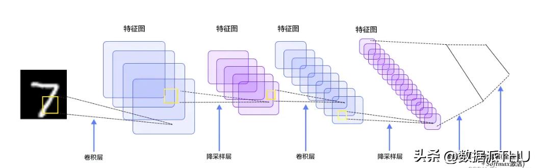
Figure 1: handwritten digital recognition process
The above process is the whole process of identifying handwritten numbers, a project that i have previously written and opened with a code that is available to interested students:
In other words, it can be seen that the entire process requires several layers of operation:
One can see that the most important of these is the volume layer, which is the origin of the name of the contours neural network, which is described in detail below。
Ii. Input layers
The input layer is relatively simple, and the main task of this layer is to enter information such as images, because the volume neural network deals mainly with the content of the images, but do we see the same images as those of the computer
It is clear that for the input of images, it is first to convert to a corresponding two-dimensional matrix, which is made up of the pixel value size of each pixel of the image. We can see an example of a handwritten number “8” image shown in the figure below, which the computer has read and stored in a two-dimensional matrix of pixel size。
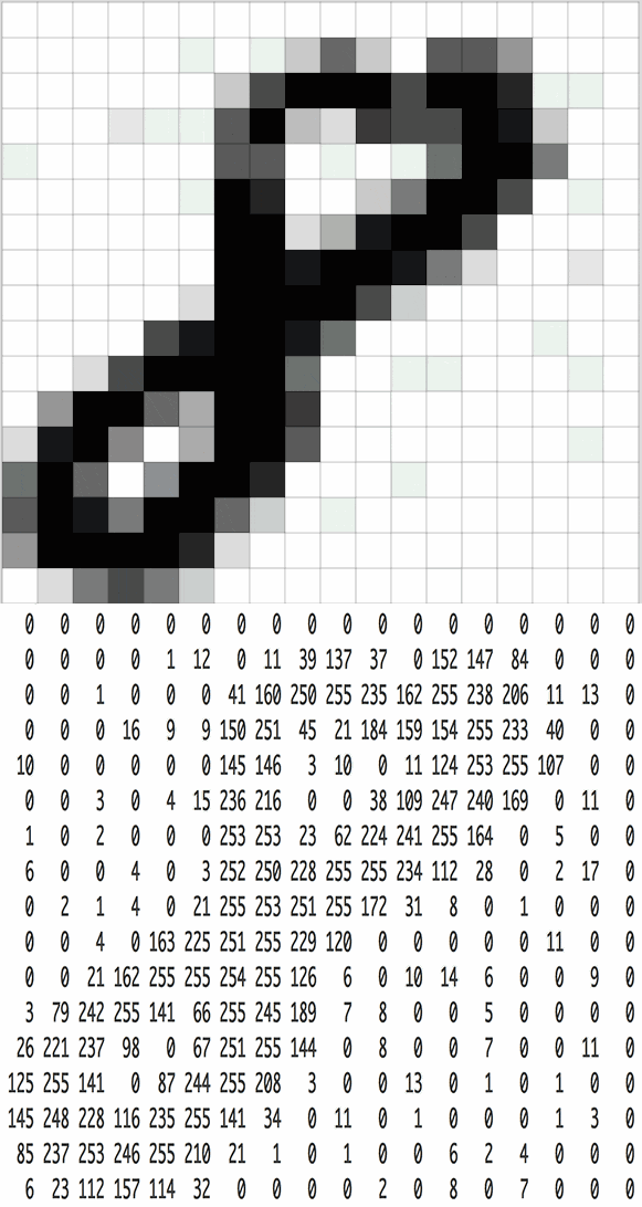
Figure 2: the two-dimensional matrix of the greyscale images of figure 8
The above figure is also referred to as a greyscale image because each of its pixel values ranges from 0 to 255 (from pure black to pure white), indicating its colour strength and weakness. There are also black and white images, with either 0 or 255 pixel values。
The most common image of our daily lives is that of rgb, with three corridors, red, green and blue. The range of pixel values per channel is also 0~255, indicating that each pixel has a strong colour。
But we're doing essentially greyscale images on a daily basis, because it's better to operate (smaller range, more single colour), and some rgb images are also converted into greyscale images before entering into the nervous network, and for easy to calculate, otherwise the pixels of the three channels together are very large。
Of course, with the rapid development of computer performance, some neural networks can now handle three-channel rgb images。
Now we know that the role of the input layer is to convert the image to its corresponding two-dimensional matrix of pixels and store the two-dimensional matrix for subsequent layers。
Volume layers
What do we do when the pictures come in
Assuming we've got the two-dimensional matrix of the picture, if we want to extract its features, the volume operation will determine a high value for the area where the characteristic exists, or a low value. It's a process that needs to be calculated by calculating it with the coThe multiplier value of nvolut kernel is determined。
Assuming that we now enter a picture of a human head, whose eyes are the characteristics we need to extract, we use the eye as a collage to determine where it is by moving on the picture of a human head, as follows:
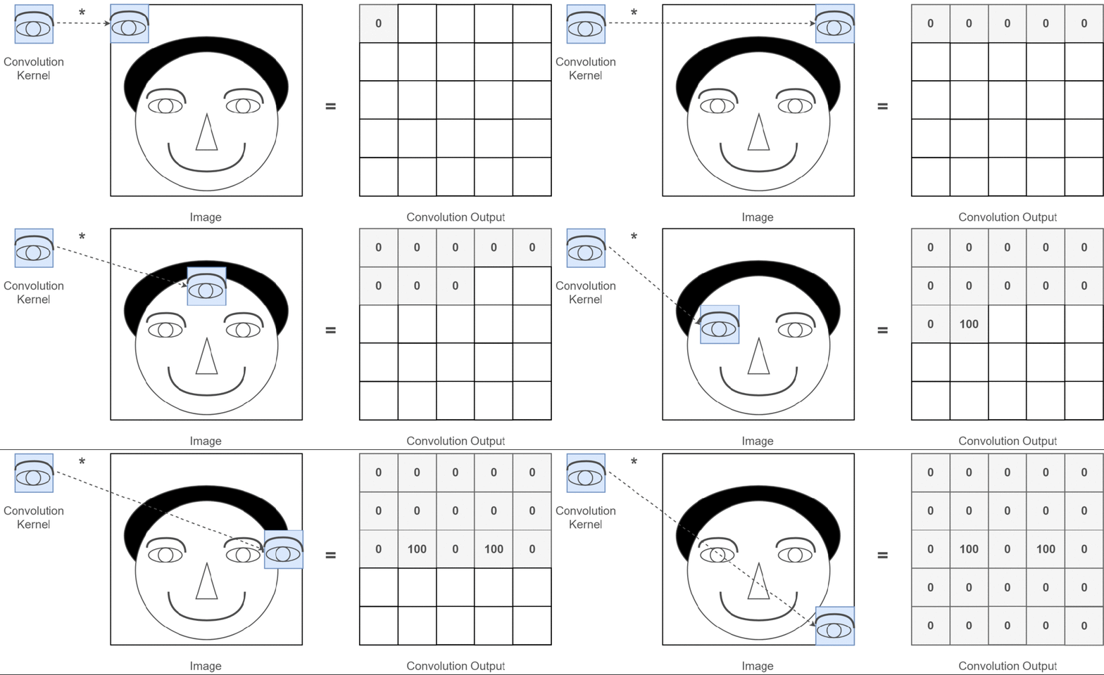
Figure 3: process of extracting human eye characteristics
A new two-dimensional matrix was obtained through the entire volume process, also known as the feature map, which, in the end, allows us to get the feature maps to be coloured (i. E., high white, low black) and finally extracts the characteristics of the eyes of a human being, as follows:
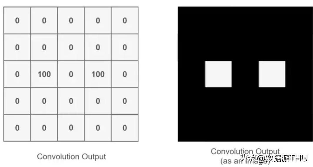
Figure 4: results of the characteristics of human eye extraction
Looking at the description above may be a bit tedious, but first, the volume core is also a two-dimensional matrix, which is, of course, smaller or more equal than the two-dimensional matrix that is inputting the image. The volume core moves constantly on the two-dimensional matrix that is inputting the image, and each move takes a multiplier sum as the value of this position, as shown in the figure below:
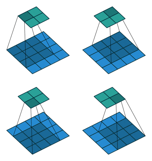
Figure 5: volume process
As you can see, the whole process is a downscaling process, which is calculated through the constant movement of a condensed core to extract the most useful features of the image。
We usually call the new two-dimensional matrix of volume core calculations a feature map, for example, in the top motion map, the dark blue square that moves below is the block core, and the green square that stays above is the feature map。
Some readers may note that the middle position is calculated every time a volume core moves, while the edge of the two-dimensional matrix of the image is calculated only once, will that result in inaccurate results
Let us think carefully that if the edges are calculated only once each time, and the middle is counted many times, the resulting feature maps also lose the marginal features and eventually lead to inaccurate character extraction, which is the solution。
We can expand around the original two-dimensional matrix of input images one or more times, so that each location can be calculated fairly and without loss of any feature. This process can be seen in the following two scenarios, which are known as padding。
• padding to one, one circle
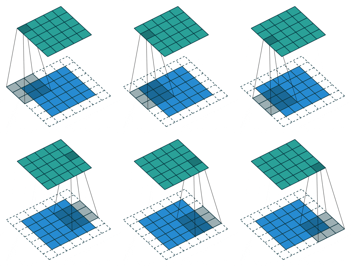
Figure 6: padding is a one-hour process
• padding to 2 with 2 rounds
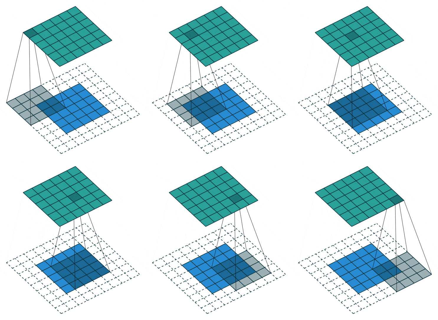
Figure 7: padding as a 2-hour volume process
What if it's more complicated? What if we use two scroll cores to extract a colored picture
As we've explained before, colour pictures are all three channels, which means that a colour picture will have three two-dimensional arrays, and of course, we'll just take the example of the first channel, or there'll be too many。
At this point, we use two sets of volume cores, each of which is used to extract the characteristics of the 2-d matrix of our own channel. As we just said, we only consider the first channel, so we only need the first set of volume cores to calculate the feature map, so the process is as follows:
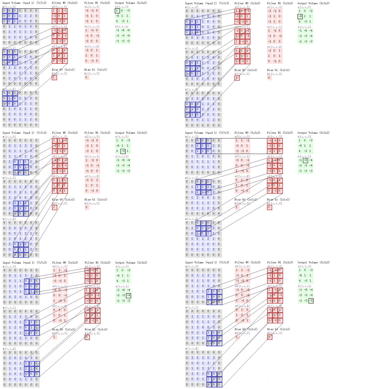
Figure 8: process of two volume cores
It's a bit confusing to look at the graph above, so let me explain, according to the way it is, the entry of the picture is colored and there are three channels, so the size of the input is 7x7x3, and we're only thinking about the first channel, which is extracting the signature from the first 7x7 2-dimensional matrix。
So all we have to do is use the first volume core in each group of volumes, and here perhaps the reader will notice bias, which is actually the bias item, and the result of the final calculation, plus it, will eventually be able to get a feature map。
It can be seen that there are several characterizations, because we now use only two graphs, so we get two graphs。
These are some of the relevant knowledge about the volume layer, and of course this is only an introduction, so there are some of the more complex elements that are not discussed in depth, and this needs to wait for later learning and summary。
Iv. Pooling
As we have also mentioned earlier, there are a few volumes of maps, and the situation is certainly more complex in reality, and there will be more maps, which, when there are so many maps, means that we have so many features, but are all the features needed
Obviously, there are a number of features that we do not need, and these redundant features usually give us two questions:
To solve this problem, we can use the pool layer. What is the pool layer
The icy layer is also referred to as subsampling, i. E., when we do a volume operation, we are able to extract the most representative of the features from the feature, which can be used to reduce the composition and dimensions, as follows:
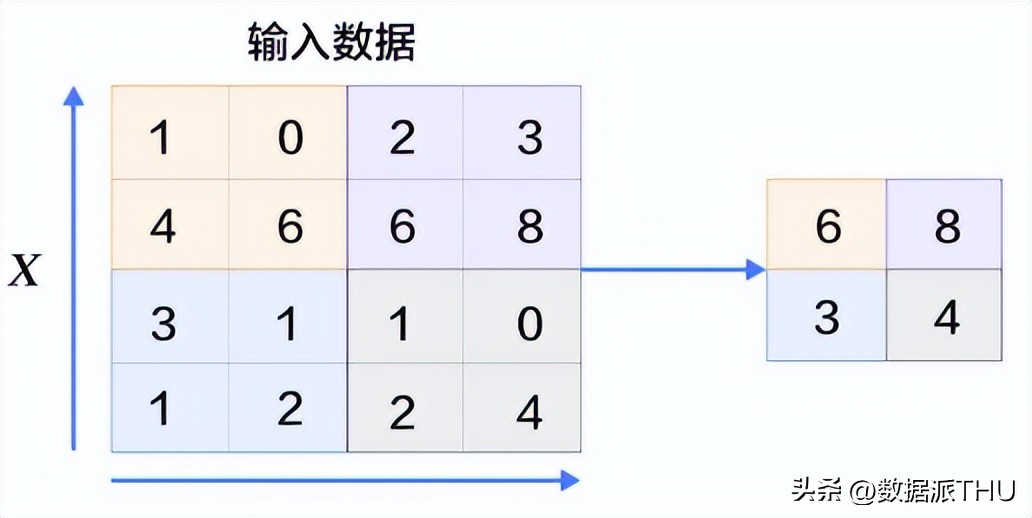
Figure 9: the process of ponding
Some readers might ask, "what rules should i use to extract?"
In fact, this process is similar to a process of volume, where a square of squares moves on a picture, and every time we take the most representative feature of this square box, then the question arises as to how to extract the most representative feature, usually in two ways:
By definition, maximum pool is the maximum value of all values in squares, which is the most representative feature of the current position, as follows:
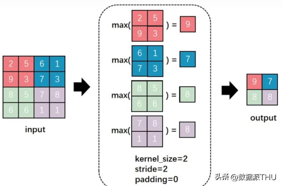
Figure 10: maximum pool process
There are several parameters to explain:
1 kernel size = 2: 2 x 2 square sizes for the pool process, indicating 2 x 2 sizes for the volume core in the process of volume
2 stride = 2: each square moves two positions (left to right, top to bottom), which is actually the same as the operation of volume
3 padding = 0: this has been introduced before, if the value is 0, it means no expansion
The average pool is the average of all values in this square area, and given the effect of the value of each position on the characteristics here, the average pool calculation is simpler, as shown in the following figure:
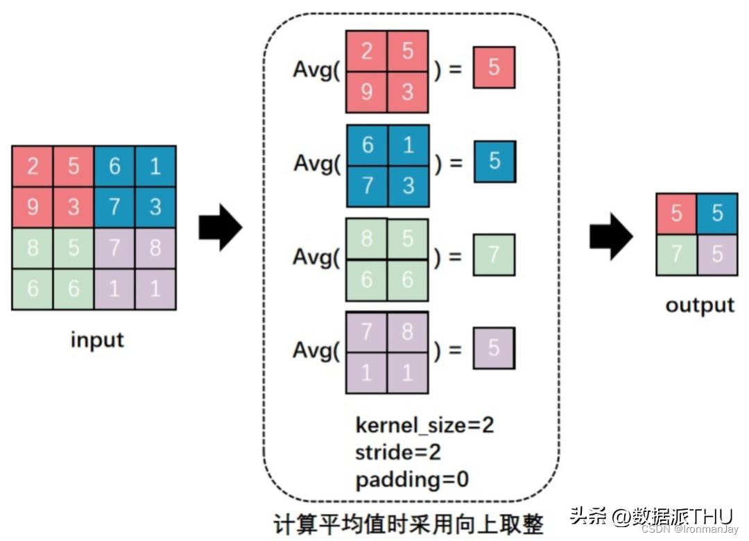
Figure 11: average pooling process
For the parameters, the meaning of which is consistent with the maximum pool described above, attention needs to be paid to the upward adjustment used in calculating the average pool。
That is all that's going on with the pool layer, and let's recall that after the pool, we can extract more representative features。
At the same time, the need for unnecessary calculations has been reduced, and this has been of great benefit to the calculation of our actual nervous network, which is very large in reality, and which, after a pool layer, can significantly increase the efficiency of the model。
So the benefits of the pool layer are many, and their advantages are summarized as follows:
These two advantages, which we have described before, are the same? An example can be drawn from our previous experience, as shown in the following figure:
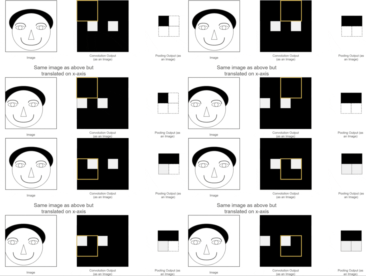
Figure 12: volatility of poolization
As you can see, two original images are different, one is normal and the other is a slight left shift in the head。
After a volume operation, the respective feature maps were obtained, and the two feature maps corresponded to the position of the original picture, with one eye feature normal and the other eye feature slightly left。
Although humans can be identified, after neuro-network calculations, errors may occur, since the place where the eyes should appear does not appear, what should be done
At this point in time, using a pool layer, it can be seen that although the eye features of the two images before the pool were not in one location, the same eye characteristics were present after the pool, which facilitated the calculation of the subsequent neural network, which is the static nature of the pool
V. Full connectivity layer
Assuming that it is also an example of the brain of the above, we have now extracted the characteristics of the person's eyes, nose and mouth through collage and collage. What if i wanted to use those characteristics to identify whether the picture was a human head
All we need to do at this point is "sizing" all the feature maps that we've extracted, turning their dimensions into 1 x 1 x 1 x 1 x x, which is a fully connected process。
That is to say, at this point, we expand and calculate all the features, and at the end we get a probabilistic value, which is the probability of whether the picture is human, as follows:
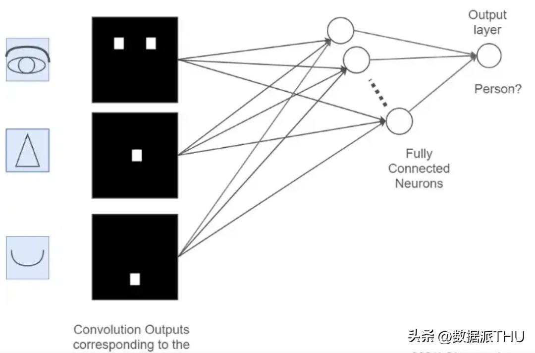
Figure 13: full connectivity process
This process may not be clear enough, so we can combine the previous process with the full connectivity layer, as shown in the figure below:
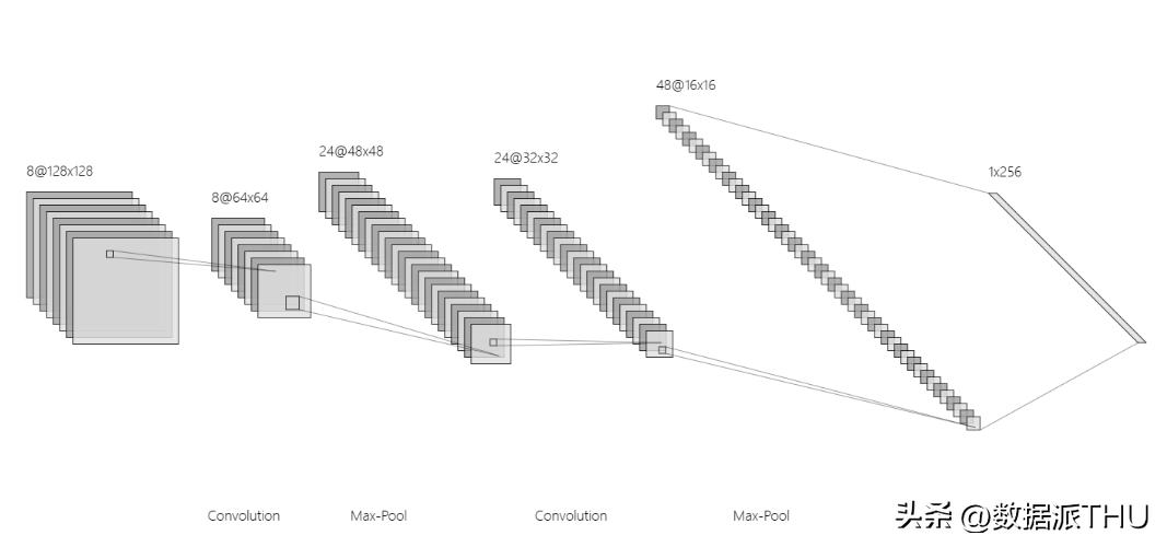
Figure 14: the whole process
As can be seen, after two volumes and maximum gestations, the final characterization was obtained, and the characteristics at this time were calculated, so they were more representative and then, after full-connected layers, they were carried out as a one-dimensional vector, and after another calculation, the ultimate recognition probability, which was the entire process of the contours neural network。
Vi. Output layer
It's easier to understand the output layers of a condensed neural network, and we just need a probability that the one-dimensional vector from the whole interconnection layer will be recognized by calculating, of course, both linear and non-linear。
In in-depth learning, the results that we need to identify are generally multi-classified, so each location has a probability value, representing the probability of being identified as current, with the maximum probability being the final recognition。
In the course of the training, the best model accuracy can be achieved by continuously adjusting parameter values to make the results more accurate。
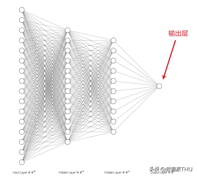
Figure 15: output layer diagram
Vii. Review of the whole process
There's no more classic use of a curly neural network than a handwritten digital recognition, like now i'm handwritten with a number eight, so how do you know that? The entire identification process is illustrated in the following figure:
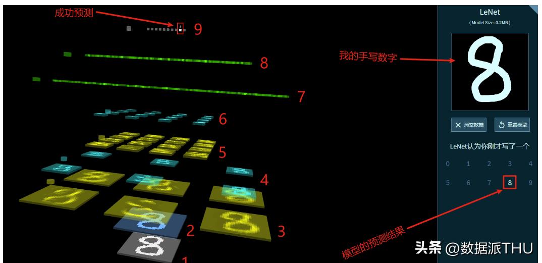
Figure 16: handwritten digital recognition process
1. Conversion of handwritten digital images into pixel matrices
2. A volume calculation of a pixel matrix that is not zero, designed to preserve a marginal feature and generate a feature figure
3. Volume calculations using six volumes for this feature map, with six features figure
4. Pooling of each feature map (also known as subsampling) to narrow the data stream while retaining the feature, generating six smaller maps, which are similar to each other, but with smaller dimensions
5. A second volume calculation of the six small maps obtained from the pool operation generated additional features figure
6. Pooling of second volume-generated feature maps (lower sampling)
7. First full connection of features from the second pool operation
8. Results of the first full connection for the second full connection
9. The final calculation of the results of the second full-link may be linear or non-linear, with a probability value for each location (a total of 10 locations, ranging from 0 to 9), that is, the probability of recognizing the handwritten number entered as the current position number and, finally, the highest probability location as the result。
As you can see, above the right is my hand-written number, below the right is the recognition of the model (lenet), and the final identification is the same as the hand-written number that i entered, as can be seen from the top left of the picture, indicating that the model can successfully identify the hand-written number。
Summary
This is all of the blog's content, and it takes me a lot of time to sum it up, hoping to learn and progress with you. Also, because of my limited skills, the reader is still in the wrong position
Original link: